
Melbourne City Area-Wise Analysis
The project aim is to analyse the geospatial data for the City of Melbourne and find their affect on house prices in that region. The datasets relating to Melbourne City’s Environment, Infrastructure and Economy are available on Open Data Melbourne, while the house selling prices were obtained from kaggle.
Firstly, we have attempted to find the good and bad areas in Melbourne in terms of the density of basic amenities available in them.
The selling prices of houses in this region can be seen in the map below.
Using Linear Regression and Random Forests, there was found to be a dependance of house prices on their proximity to a few of those amenities. Linear Regression’s results, being more easily interpretable, show the magnitude of dependance of each variable on the Price.
| Variable | Coefficient |
|---|---|
| tree_distance | 84.04 |
| light_distance | -57.88 |
| palyg_distance | 168.73 |
| featurelight_distance | 77.21 |
| Rooms | 454965.97 |
| height | -1370.60 |
| metro_distance | 150.33 |
| syringebin_distance | -192.58 |
| cafe_distance | -39.99 |
| bar_distance | -157.00 |
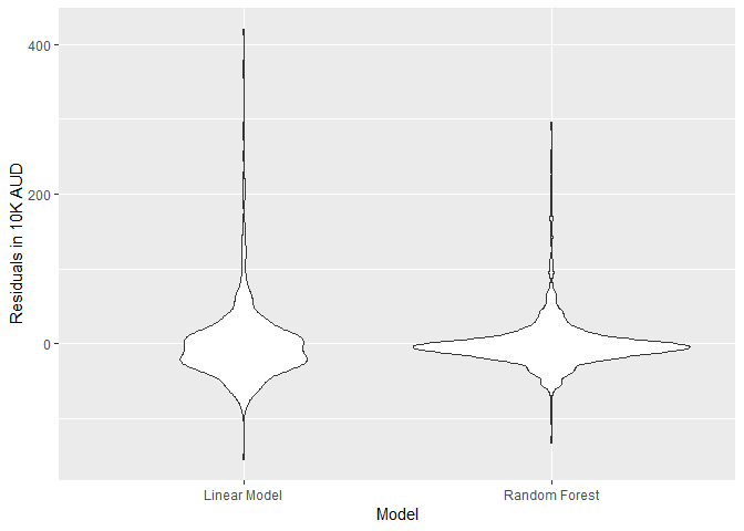
Random Forests, being an ensemble learning technique, gave better results as can be seen in the following violin plot showing the distribution of residuals obtained from both algorithms.
The scatter plot of the actual vs predicted price shows that our RF model is pretty accurate.
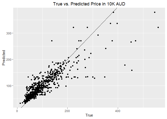
For some houses, there is a significant difference between their actual selling price and the price our model predicts they should be sold for. Based on this observation, these houses can be grouped into undervalued and overvalued.The map shows the price residuals; the ones with most negative residuals are undervalued and are a good deals for home-seekers.The ones with most positive residuals are overvalued and cost more than what the model predicts.
Visit the Github Repository here.